Seeyong's Blog
파일에서 데이터 읽어오기
실제 데이터 분석을 할 때는 매번 직접 데이터를 입력하기 보다 기존에 있는 파일을 읽어오는 경우가 많다. 파일에서 데이터를 읽어와 학습을 해보자.
import numpy as np
xy = np.loadtxt('data-01-test-score.csv', delimiter=',', dtype=np.float32)
x_data = xy[:, 0:-1]
y_data = xy[:, [-1]]
numpy 라이브러리를 사용해서 파일을 읽어올 수 있다.csv 파일이기 때문에 delimiter 값을 ,로 지정해두고 data type은 float으로 읽어온다. 그리고 slicing을 통해 x_data와 y_data의 node를 분류한다.
# Make sure the shape and data are OK
print(x_data.shape, len(x_data))
x_data[:10]
x_data의 형태를 살펴보면,
(25, 3) 25
array([[ 73.,  80.,  75.],
       [ 93.,  88.,  93.],
       [ 89.,  91.,  90.],
       [ 96.,  98., 100.],
       [ 73.,  66.,  70.],
       [ 53.,  46.,  55.],
       [ 69.,  74.,  77.],
       [ 47.,  56.,  60.],
       [ 87.,  79.,  90.],
       [ 79.,  70.,  88.]], dtype=float32)
다음과 같고, 마찬가지로 y_data의 형태는 아래와 같이 확인할 수 있다.
print(y_data.shape)
y_data[:10]
(25, 1)
array([[152.],
       [185.],
       [180.],
       [196.],
       [142.],
       [101.],
       [149.],
       [115.],
       [175.],
       [164.]], dtype=float32)
이제부터는 기존의 방식대로 Hypothesis와 cost 함수를 만들어 학습을 시키면 된다.
# placeholders for a tensor that will be always fed.
X = tf.placeholder(tf.float32, shape=[None, 3])
Y = tf.placeholder(tf.float32, shape=[None, 1])

W = tf.Variable(tf.random_normal([3, 1]), name='weight')
b = tf.Variable(tf.random_normal([1]), name='bias')

# Hypothesis
hypothesis = tf.matmul(X, W) + b

# Simplified cost/loss fuction
cost = tf.reduce_mean(tf.square(hypothesis - Y))

# Minimize
optimizer = tf.train.GradientDescentOptimizer(learning_rate=1e-5)
train = optimizer.minimize(cost)

# Launch the graph in a session
sess = tf.Session()

# Initializes global variable in the graph
sess.run(tf.global_variables_initializer())

# Set up feed_dict variables in the loop
for step in range(2001):
    cost_val, hy_val, _ = sess.run(
    [cost, hypothesis, train],
    feed_dict={X: x_data, Y: y_data})
학습을 시킨 후 임의의 점수를 x_data로 집어 넣어보자.
# Ask my score
print('Your Score will be ', '%.10f' % sess.run(hypothesis,
                                     feed_dict={X: [[100, 70, 101]]}))

print('Other Score will be ', sess.run(hypothesis,
                                      feed_dict={X: [[60, 70, 110], [90, 100, 80]]}))
x_data의 차원만 일치한다면 몇개의 데이터가 입력되어도 학습 후 결과를 나타낼 수 있다.
Your Score will be  191.4561004639
Other Score will be  [[187.48228], [172.1105 ]]
위와 같이 학습한 결과를 도출해낼 수 있다.
여러 파일 읽어오기
하지만 파일 하나만 읽어오는 경우 뿐 아니라 여러 파일을 동시에 읽어와야 하는 경우도 있다. 데이터의 크기가 크거나, 다른 종류(ex)다른 마케팅 채널 등)의 데이터를 동시에 분석해야 할 때가 있다. 이를 위해 TensorFlow에서 파일을 어떻게 처리하는지 살펴볼 필요가 있다.
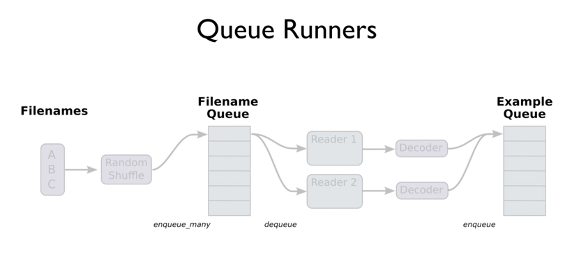

1 여러개의 파일을 하나의 Queue로 만들기
filename_queue = tf.train.string_input_producer(
    ['data-01-test-score.csv'], shuffle=False, name='filename_queue')
string_input_producer 메소드를 사용해 여러개의 파일을 입력하고 shuffle 여부와 queue의 이름을 지정한다.
2 해당 Queue를 Read하기
reader = tf.TextLineReader()
key, value = reader.read(filename_queue)
TextLineReader를 사용해 key와 value를 가져온다.
3 읽어온 데이터를 Decode하기
record_defaults = [[0.], [0.], [0.], [0.]]
xy = tf.decode_csv(value, record_defaults=record_defaults)

# collect batches of csv in
train_x_batch, train_y_batch = tf.train.batch([xy[0:-1], xy[-1:]], batch_size=10)
읽어오는 파일 데이터의 차원과 데이터 타입을 지정해두고 value 값을 decode해서 xy라는 새로운 node에 바인딩한다. 이후 train_x_batch와 train_y_batch의 큰 뭉치를 각각 만들어낸다. batch_size도 지정할 수 있다. 이후는 기존의 학습 방식과 동일하다.
# placeholders for a tensor that will be always fed.
X = tf.placeholder(tf.float32, shape=[None, 3])
Y = tf.placeholder(tf.float32, shape=[None, 1])

W = tf.Variable(tf.random_normal([3, 1]), name='weight')
b = tf.Variable(tf.random_normal([1]), name='bias')

# Hypothesis
hypothesis = tf.matmul(X, W) + b

# Simplified cost/loss fuction
cost = tf.reduce_mean(tf.square(hypothesis - Y))

# Minimize
optimizer = tf.train.GradientDescentOptimizer(learning_rate=1e-5)
train = optimizer.minimize(cost)
Hypothesis와 cost 함수를 지정해둔 후,
# Launch the graph in a session
sess = tf.Session()

# Initializes global variable in the graph
sess.run(tf.global_variables_initializer())

# Start populating the filename_queue
coord = tf.train.Coordinator()
threads = tf.train.start_queue_runners(sess=sess, coord=coord)

# Set up feed_dict variables in the loop
for step in range(2001):
    x_batch, y_batch = sess.run([train_x_batch, train_y_batch])
    cost_val, hy_val, _ = sess.run(
        [cost, hypothesis, train], feed_dict={X: x_batch, Y: y_batch})

coord.request_stop()
coord.join(threads)

# Ask my score
print("Your score will be ",
      sess.run(hypothesis, feed_dict={X: [[100, 70, 101]]}))

print("Other scores will be ",
      sess.run(hypothesis, feed_dict={X: [[60, 70, 110], [90, 100, 80]]}))
각 batch를 feed_dict에 알맞은 형태로 넣어서 학습을 시키면 된다.
Your score will be  [[191.81798]]
Other scores will be  [[195.14287], [169.19527]]
이렇게 결과값이 도출된다. 재밌는 사실은 동일하게 2,000 번 반복하며 학습을 했지만 앞선 결과값과는 조금 다른 숫자가 나왔다는 사실이다.