Seeyong's Blog
0 또는 1
그동안 학습해온 TensorFlow는 시험 점수 처럼 제한 없는 미지의 특정 값을 예측하는 데에 사용되었다. 하지만 이런 경우는 어떨까. Pass와 Non-pass로 결과를 나누는 시험이라든가 쇼핑몰에서 고객이 물건을 살지 안살지를 판가름해야 하는 경우. 시험 점수를 도출해내듯이 예측하기 어렵다. 이제 우리는 새로운 Hypothesis를 세워야 한다.
Logistic (regression) Classifier
그동안의 선형회귀(Linear Regression)에서는 밥그릇을 거꾸로 엎어놓은 형태의 그래프를 수식으로 표현의 우리의 가설로 사용했다. 하지만 최종적으로 0과 1을 구분하기 위한 가설 검증에는 적용하기 어려운 몇가지 이유가 있다. 수학적인 이야기는 메인 주제에서 벗어나기 때문에 결과적으로 어떤 형태의 가설을 사용하는지 살펴보자.

sigmoid function이라고 부르는 수식을 수학자들이 이미 만들어 놨다. 우리는 이 공식을 코드에 적용하기만 하면 된다. 앞서 말했듯 새로운 Hypothesis를 사용하는 이유는 0과 1이라는 두개의 값만 도출해내기 위해서이다.
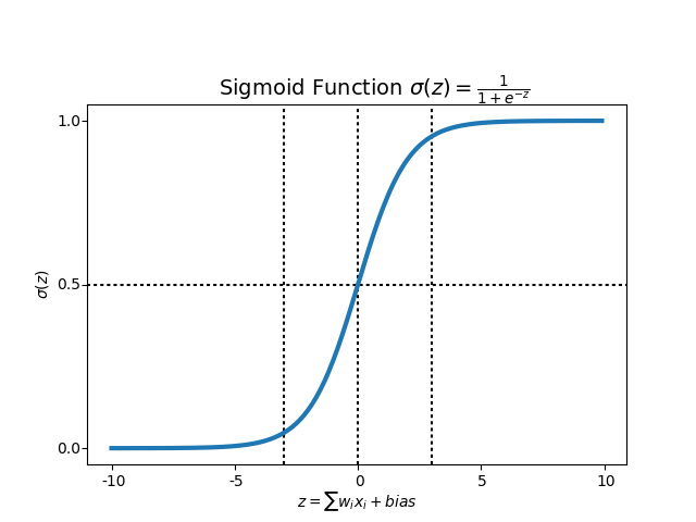 수식을 그래프로 나타내면 이런 모습이다. 아무리
 Data가 크거나 작아져도 0과 1 사이를 벗어나지 않는다. 우리가 원하는 모양이다.

자연스럽게 cost의 수식도 달라진다. 이 역시 자세한 수학적인 논리보다 결과식을 살펴보자. 크게 두가지 경우로 나눠볼 수 있다. 실제 Y값이 0일 때와 1일 때의 각 cost의 평균을 구하는 공식이다. Y = 0일 경우 앞의 log함수가 없어지고, Y = 1일 경우 뒤의 log함수가 없어지므로 각 경우마다 단 하나의 cost 값만 남게 된다. 즉, Data의 숫자만큼 결과값을 학습할 수 있다.

새로운 cost함수를 미분하면 위의 식이 된다. cost 함수는 다시금 엎어놓은 밥그릇 모양이 되었기 때문에 그 기울기를 구하면서 가장 낮은 수준의 cost를 찾아 학습할 수 있다.
Training Data
import tensorflow as tf

x_data = [[1,2], [2,3], [3,1], [4,3], [5,3], [6,2]]
y_data = [[0], [0], [0], [1], [1], [1]]

X = tf.placeholder(tf.float32, shape=[None, 2])
Y = tf.placeholder(tf.float32, shape=[None, 1])

W = tf.Variable(tf.random_normal([2,1]), name='weight')
b = tf.Variable(tf.random_normal([1]), name='bias')
이제 실제 코드로 구현해보자. x_data는 기존과 같이 대입되지만 y_data는 0 또는 1의 형태로 도출되는 것을 볼 수 있다.
# Hypothesis using sigmoide: tf.div(1., 1. + tf.exp(tf.matmul(X, W)) + b)
hypothesis = tf.sigmoid(tf.matmul(X, W) + b)

# cost/loss function
cost = -tf.reduce_mean(Y * tf.log(hypothesis) + (1 - Y) * tf.log(1 - hypothesis))

train = tf.train.GradientDescentOptimizer(learning_rate=0.01).minimize(cost)

# Accuracy computation
# True if hypothesis > 0.5 else False
predicted = tf.cast(hypothesis > 0.5, dtype=tf.float32)
accuracy = tf.reduce_mean(tf.cast(tf.equal(predicted, Y), dtype=tf.float32))
이제 우리는 hypothesis에 새로운 공식을 대입한다. 우리가 직접 위의 공식을 하나하나 대입할 필요 없이 TensorFlow에서 이미 sigmoid 메소드를 만들어놨다. 사용만 하면 된다. cost 함수도 새롭게 구현을 한다.
이제 우리는 predicted라는 node에 cast 메소드를 사용해 우리의 가설에 의해 도출된 예측 값이 0.5를 넘는지 판단한다. 넘을 경우 1로 간주하고 반대일 경우 0으로 간주하는 방식이다.
Train the model
# Launch graph
with tf.Session() as sess:
    # Initialize TensorFlow Variables
    sess.run(tf.global_variables_initializer())

    for step in range(10001):
        cost_val, _ = sess.run([cost, train], feed_dict={X: x_data, Y: y_data})
        if step % 1000 == 0:
            print(step, cost_val)

    # Accuracy report
    h, c, a = sess.run([hypothesis, predicted, accuracy],
                  feed_dict={X: x_data, Y: y_data})
    print("\nHypothesis: ", h, "\nCorrect (Y): ", c, "\nAccuracy: ", a)
feed_dict에 각각 x_data와 y_data를 대입해서 학습을 시키고, hypothesis와 predicted, accuracy를 알아볼 수 있다.
0 2.157367
1000 0.34064794
2000 0.29229894
3000 0.2563405
4000 0.22776479
5000 0.20464057
6000 0.18564326
7000 0.169814
8000 0.15645158
9000 0.14503819
10000 0.13518567

Hypothesis:
[[0.02495899]
 [0.15018529]
 [0.2758761 ]
 [0.79495776]
 [0.94780606]
 [0.98296505]]
Correct (Y):
[[0.]
 [0.]
 [0.]
 [1.]
 [1.]
 [1.]]
Accuracy:  1.0
소규모의 명확한 data들을 학습시켰기 때문에 accuracy가 100%로 나왔다. 하지만 현실 데이터를 사용할 경우 그 정확도는 떨어지기 마련이다.
import numpy as np

xy = np.loadtxt('data-03-diabetes.csv', delimiter=',', dtype=np.float32)
x_data = xy[:, 0:-1]
y_data = xy[:, [-1]]
실제 당뇨병 검사 결과와 여러 feature를 정리한 데이터를 가져와서 학습을 진행해보자.
X = tf.placeholder(tf.float32, shape=[None, 8])
Y = tf.placeholder(tf.float32, shape=[None, 1])

W = tf.Variable(tf.random_normal([8,1]), name='weight')
b = tf.Variable(tf.random_normal([1]), name='bias')

# Hypothesis using sigmoide: tf.div(1., 1. + tf.exp(tf.matmul(X, W)) + b)
hypothesis = tf.sigmoid(tf.matmul(X, W) + b)

# cost/loss function
cost = -tf.reduce_mean(Y * tf.log(hypothesis) + (1 - Y) * tf.log(1 - hypothesis))

train = tf.train.GradientDescentOptimizer(learning_rate=0.01).minimize(cost)

# Accuracy computation
# True if hypothesis > 0.5 else False
predicted = tf.cast(hypothesis > 0.5, dtype=tf.float32)
accuracy = tf.reduce_mean(tf.cast(tf.equal(predicted, Y), dtype=tf.float32))

# Launch graph
with tf.Session() as sess:
    # Initialize TensorFlow Variables
    sess.run(tf.global_variables_initializer())

    for step in range(10001):
        cost_val, _ = sess.run([cost, train], feed_dict={X: x_data, Y: y_data})
        if step % 1000 == 0:
            print(step, cost_val)

    # Accuracy report
    h, c, a = sess.run([hypothesis, predicted, accuracy],
                  feed_dict={X: x_data, Y: y_data})
    print("\nHypothesis: ", h, "\nCorrect (Y): ", c, "\nAccuracy: ", a)
앞서 소규모 데이터의 사례와 마찬가지 과정을 거치지만 각 분석마다 x_data의 차원, 그리고 이에 따라 달라지는 weight의 차원을 함께 고려해서 조정해줘야 한다. 여기서는 x_data가 가지고 있는 feature의 개수가 8개이므로 차원을 조정해주었다.
0 1.6834059
1000 0.67501724
2000 0.6000349
3000 0.5585303
4000 0.5339053
5000 0.5182685
6000 0.5077621
7000 0.5003763
8000 0.49499282
9000 0.4909516
10000 0.48784316

Hypothesis:
[[0.40653372]
 [0.91259897]
 [0.29548234]
 [0.93671775]
 [0.27462035]
 [0.7768192 ]
 ...
 [0.75612897]
 [0.6890358 ]
 [0.806679  ]
 [0.77790445]
 [0.87626946]]
Correct (Y):
[[0.]
 [1.]
 [0.]
 [1.]
 [0.]
 ...
 [0.]
 [1.]
 [1.]
 [1.]
 [1.]
 [1.]
 [1.]]
Accuracy:  0.77470356
accuracy가 0.77 수준으로 떨어진 것을 확인할 수 있다. data의 숫자가 많아질 수록 정확도가 떨어질 수 밖에 없으므로 y_data를 잘 설명해주는 feature를 논리적으로 선정하는 방법과 학습을 시킬 수 있는 sample 숫자를 적정 수준 이상으로 학습을 진행하는 방법이 필요하다.