Seeyong's Blog
Use MATRIX!
Multi-variable Linear Regression
Hypothesis using Matrix
그동안 \($x\)$라는 feature가 하나인 간단한 선형 회귀 분석을 해왔지만 현실에는 여러개의 feature가 있는 경우가 대부분이다. 이제 우리는 여러개의 \($x\)$를 사용해 회귀 분석을 하고 예측치를 도출할 것이다.
student|Quiz 1(\($x_1\)$)|Midterm(\($x_2\)$)|Quiz 2(\($x_3\)$)|Final(\($y\)$)
——-|——|——|——-|——
A|73|80|75|152
B|93|88|93|185
C|89|91|90|180
D|96|98|100|196
E|73|66|70|142
위와 같이 5명의 학생들 퀴즈와 중간고사 성적, 그리고 기말고사 성적이 기록되어 있다. 이 점수를 가지고 학생들의 퀴즈, 중간고사 성적만 가지고 기말고사 점수를 예측하는 학습을 실행할 것이다.
import tensorflow as tf

x1_data = [73.,93.,89.,96.,73.]
x2_data = [80.,88.,91.,98.,66.]
x3_data = [75.,93.,90.,100.,70.]
y_data = [152.,185.,180.,196.,142.]

# placeholders for a tensor that will be always fed
x1 = tf.placeholder(tf.float32)
x2 = tf.placeholder(tf.float32)
x3 = tf.placeholder(tf.float32)

Y = tf.placeholder(tf.float32)

w1 = tf.Variable(tf.random_normal([1]), name='weight1')
w2 = tf.Variable(tf.random_normal([1]), name='weight2')
w3 = tf.Variable(tf.random_normal([1]), name='weight3')
b = tf.Variable(tf.random_normal([1]), name='bias')

hypothesis = x1 * w1 + x2 * w2 + x3 * w3 + b
표에서 구성되어 있는 각 column들 하나하나가 y라는 기말고사 점수를 예측하는 feature로 사용된다. 그렇기 때문에 일단 학생 단위가 아닌 feature단위로 x_data를 만들었다.
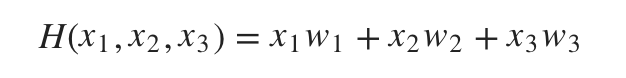
우리의 Hypothesis 식에서 b=0으로 가정하고 나면 아래와 같은 식이 도출된다.
\(H(x_1, x_2, x_3) = x_1w_1 + x_2w_2 + x_3w_3\)
 각
각 w는 1차원으로 구성된 weight이기 때문에 Variable로 지정한 뒤 hypothesis라는 node에 가설식을 구현한다.
# cost/loss function
cost = tf.reduce_mean(tf.square(hypothesis - Y))
# Minimize. Need a very small learing rate for this data set
optimizer = tf.train.GradientDescentOptimizer(learning_rate=1e-5)
train = optimizer.minimize(cost)

# Launch the graph in a session
sess = tf.Session()
# Initializes global variables in the graph
sess.run(tf.global_variables_initializer())
for step in range(20001):
    cost_val, hy_val, _ = sess.run([cost, hypothesis, train],
                                  feed_dict={x1: x1_data, x2: x2_data, x3: x3_data, Y: y_data})
    if step % 1000 == 0:
        print(step, "Cost :", cost_val, "Prediction :", hy_val)
cost를 구현한 뒤 아주 작은 수의 learning_rate를 지정해 GradientDescentOptimizer를 학습시키도록 한다. 20000번 동안 cost, hypothesis를 실행하고 1000번 마다 출력하면 아래와 같은 결과가 나온다.
0 Cost : 59467.523 Prediction : [-77.99535  -66.57198  -79.89152  -82.39722  -48.007053]
1000 Cost : 41.099026 Prediction : [141.03563 191.45213 177.07451 197.02803 147.83372]
2000 Cost : 25.257984 Prediction : [143.1631  190.00246 177.73758 197.42075 146.00468]
3000 Cost : 15.984553 Prediction : [144.79411 188.89296 178.24826 197.70525 144.62038]
4000 Cost : 10.5335045 Prediction : [146.0463  188.04291 178.64261 197.90756 143.5749 ]
5000 Cost : 7.3084106 Prediction : [147.00935 187.39087 178.9481  198.04753 142.78764]
6000 Cost : 5.3804464 Prediction : [147.75177 186.88995 179.18576 198.14034 142.19705]
7000 Cost : 4.2093663 Prediction : [148.32568 186.5043  179.37155 198.19748 141.7562 ]
8000 Cost : 3.4808178 Prediction : [148.77095 186.20668 179.51767 198.22777 141.42934]
9000 Cost : 3.0119166 Prediction : [149.11792 185.9763  179.63348 198.23792 141.18918]
10000 Cost : 2.6961677 Prediction : [149.38971 185.79723 179.72597 198.23296 141.01488]
11000 Cost : 2.4715145 Prediction : [149.60403 185.65741 179.80067 198.21683 140.89064]
12000 Cost : 2.301794 Prediction : [149.77435 185.54758 179.86166 198.19246 140.80434]
13000 Cost : 2.165877 Prediction : [149.91093 185.46071 179.9121  198.1621  140.74678]
14000 Cost : 2.0513682 Prediction : [150.02162 185.3914  179.9544  198.12743 140.71095]
15000 Cost : 1.9510012 Prediction : [150.11246 185.33562 179.99042 198.08981 140.69151]
16000 Cost : 1.8604387 Prediction : [150.18794 185.29015 180.02155 198.05014 140.68436]
17000 Cost : 1.7771279 Prediction : [150.2516  185.25264 180.04884 198.00922 140.68639]
18000 Cost : 1.699481 Prediction : [150.30606 185.22128 180.07314 197.96756 140.69525]
19000 Cost : 1.6264855 Prediction : [150.35344 185.1947  180.0951  197.92564 140.70918]
20000 Cost : 1.5575465 Prediction : [150.39519 185.17177 180.11513 197.88371 140.72675]
cost는 게속해서 줄어들고 학습된 가설의 결과물도 실제 기말고사(Y) 값과도 가까워진다. 여러 변수를 선형 회귀 분석식에 넣어 학습이 잘 되었다는 결론이다.
Matrix
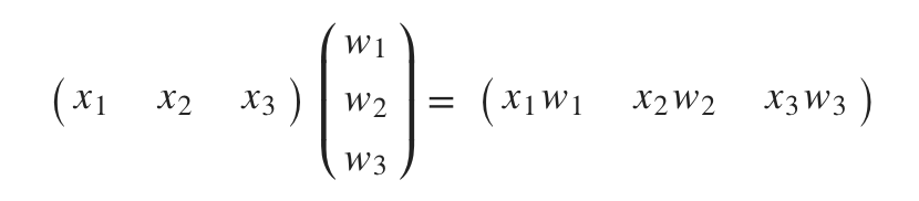
그런데 feature의 개수가 수도 없이 많아지면 어떻게 해야할까. 매번 하나하나 변수를 지정할 수 없다. 이를 해결하기 위해 이제부터 행렬(Matrix)을 사용할 것이다.
\(\left(\begin{array}{cc}
x_1 & x_2 & x_3\\
\end{array}\right)
\left(\begin{array}{cc}
w_1\\
w_2\\
w_3
\end{array}\right)
=
\left(\begin{array}{cc}
x_1w_1 & x_2w_2 & x_3w_3\\
\end{array}\right)\)
 중학생 때 배운
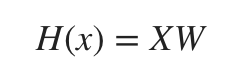
 행렬의 곱셉을 사용하면 선형 회귀 가설식을 간단하게 도출할 수 있다. 함축된 식으로 다시 정리해보면,
\(H(x) = XW\)
 대문자로 표시된 각
 X와 W는 행렬(Matrix)이라는 의미다.
x_data = [[73.,80.,75.],[93.,88.,93.],[89.,91.,90.],[96.,98.,100.],[73.,66.,70.]]
y_data = [[152.],[185.],[180.],[196.],[142.]]
이제 x_data라는 변수 안에는 각 학생별 점수가 리스트의 형태로 담겨져있다. 행렬로 표시할 수 있다는 의미다.
y_data역시 최종적인 결과물인 기말고사 점수를 행렬의 형태로 담고 있다.
# placeholders for a tensor that will be always fed
X = tf.placeholder(tf.float32, shape=[None, 3])
Y = tf.placeholder(tf.float32, shape=[None, 1])

W = tf.Variable(tf.random_normal([3, 1]), name='weight')
b = tf.Variable(tf.random_normal([1]), name='bias')
우리가 행렬을 능숙하게 사용하기 위해서는 행렬이 어떤 형태로 이뤄져있는지 알고 있어야 한다. 먼저 x_data는 5 X 3의 형태다. 5개의 instance(학생 수)가 있고 각 학생이 3번의 feature(시험점수)를 가지고 있기 때문이다. feature와 instance의 개수가 늘어나고 줄어듬에 따라 행렬의 모양은 변한다.
y_data는 5 X 1의 형태다. 학생수라는 instance의 개수, 도출되는 결과값(Y)의 개수로 이뤄져있기 때문이다. 이를 코드로 표현하면 위 코드와 같다. None은 값이 없다는 의미가 아니라 N개의 instance를 가지고 있다는 의미로 이해할 수 있다.
(5 X 3) 행렬를 다른 어떤 행렬과 곱해 (5 X 1) 형태의 행렬로 만들기 위해서는 가운데 또 하나의 행렬이 필요하다.
\((5 \times 3) \times (i \times j) = (5 \times 1)\)
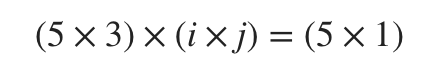
i는 3이 되어야 하고 j는 1이 되어야 결과값이 완성된다. 즉, \($H(x) = XW\)$에서 W는 (3 X 1)의 형태가 되어야 한다.
# Hypothesis
hypothesis = tf.matmul(X, W) + b
# cost/loss function
cost = tf.reduce_mean(tf.square(hypothesis - Y))
# Minimize. Need a very small learing rate for this data set
optimizer = tf.train.GradientDescentOptimizer(learning_rate=1e-5)
train = optimizer.minimize(cost)

# Launch the graph in a session
sess = tf.Session()
# Initializes global variables in the graph
sess.run(tf.global_variables_initializer())
for step in range(20001):
    cost_val, hy_val, _ = sess.run([cost, hypothesis, train],
                                  feed_dict={X: x_data, Y: y_data})
    if step % 1000 == 0:
        print(step, "Cost :", cost_val, "Prediction :", hy_val)
hypothesis 공식은 행렬 X와 행렬 W의 곱으로 간단하게 나타낼 수 있다. 역시 20000의 학습을 거치고 1000번 마다 결과값을 출력해보면 아래와 같다.
0 Cost : 151066.53 Prediction : [[-193.82428]
 [-229.79375]
 [-228.08527]
 [-246.60347]
 [-176.2027 ]]
1000 Cost : 1.8139706 Prediction : [[150.90787]
 [184.81007]
 [180.2997 ]
 [198.07117]
 [140.1395 ]]
2000 Cost : 1.688638 Prediction : [[150.81036]
 [184.88274]
 [180.27719]
 [197.99756]
 [140.28328]]
3000 Cost : 1.5897057 Prediction : [[150.74161]
 [184.93552]
 [180.26329]
 [197.93156]
 [140.39983]]
4000 Cost : 1.5073559 Prediction : [[150.69464]
 [184.97325]
 [180.25592]
 [197.87163]
 [140.49547]]
5000 Cost : 1.4358529 Prediction : [[150.66415]
 [184.99954]
 [180.25343]
 [197.81654]
 [140.57497]]
6000 Cost : 1.3717347 Prediction : [[150.64615]
 [185.01718]
 [180.25458]
 [197.76538]
 [140.64203]]
7000 Cost : 1.312979 Prediction : [[150.6375 ]
 [185.02824]
 [180.25845]
 [197.7174 ]
 [140.69946]]
8000 Cost : 1.2583884 Prediction : [[150.63586]
 [185.03436]
 [180.26431]
 [197.6721 ]
 [140.74936]]
9000 Cost : 1.2071766 Prediction : [[150.63945]
 [185.03679]
 [180.2716 ]
 [197.62903]
 [140.79338]]
10000 Cost : 1.158845 Prediction : [[150.64693]
 [185.03642]
 [180.27995]
 [197.58788]
 [140.8328 ]]
11000 Cost : 1.1130654 Prediction : [[150.65724]
 [185.03401]
 [180.28902]
 [197.54837]
 [140.86855]]
12000 Cost : 1.0696104 Prediction : [[150.66963]
 [185.03008]
 [180.29857]
 [197.51033]
 [140.90135]]
13000 Cost : 1.0282876 Prediction : [[150.68349]
 [185.02504]
 [180.30846]
 [197.47359]
 [140.93182]]
14000 Cost : 0.9890025 Prediction : [[150.69832]
 [185.01918]
 [180.3185 ]
 [197.43803]
 [140.96034]]
15000 Cost : 0.95158184 Prediction : [[150.71385]
 [185.01277]
 [180.32861]
 [197.40353]
 [140.98724]]
16000 Cost : 0.91597384 Prediction : [[150.72977]
 [185.00598]
 [180.33871]
 [197.37006]
 [141.0128 ]]
17000 Cost : 0.88204765 Prediction : [[150.74593]
 [184.99895]
 [180.34877]
 [197.33752]
 [141.03723]]
18000 Cost : 0.84974307 Prediction : [[150.76213]
 [184.99178]
 [180.35872]
 [197.30586]
 [141.06065]]
19000 Cost : 0.81897116 Prediction : [[150.77829]
 [184.98453]
 [180.36853]
 [197.27502]
 [141.08319]]
20000 Cost : 0.7896425 Prediction : [[150.79436]
 [184.97728]
 [180.3782 ]
 [197.24501]
 [141.105  ]]
cost는 더욱 많이 줄어들고 결과값도 실제 Y값과 더 근접해졌음을 확인할 수 있다. 이제 우리는 여러 변수가 있더라도 행렬(Matrix)을 사용해 간단하게 학습을 할 수 있다.